Create a Pivot Table

Excel Tutorial

Create a pivot Table

How to create a Pivot Table in Excel

Solution of this problem.
Make a data with columns containing Product, Sales 2015 and Sales 2016


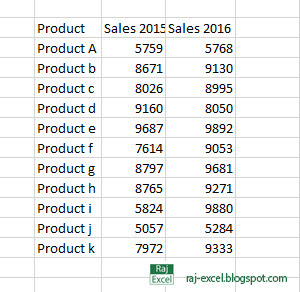
Note: The best way to get the selection of data please make sure the data should be in table form. If you want to update or extend your data. Range of the data will automatically extend.
If you do not need to extend your data, you can direct by select as a range.

To create a table, select the data and press Ctrl + T

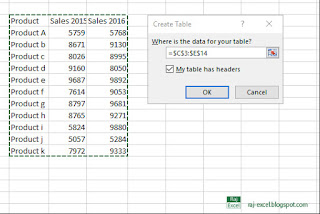
and check the My table has header and then click OK.
If you don’t check the My table has headers box, table headers with default names like Column1 and Column2 are added to your table above its data. You can change default header names at any time.
 



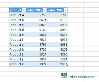
When you convert your data to table form now you will see that after the last tab of ribbon new tab “Design” table tools will be visible in ribbon.




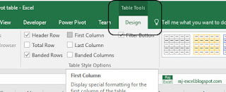
Select the design tab and on left side of tab select the “Summarize with the Pivot Table”.




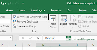
New popup window “Create Pivot Table” will appear on screen. Select Table/Range. In default selection you will see the table name “Table1”. You can use the external data as well.




 
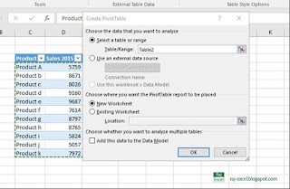
Now select the area you want to view your data/Pivot Table. Select the New Worksheet and then click OK.
In 2016 there is new option for “Add this data to the Data Model”


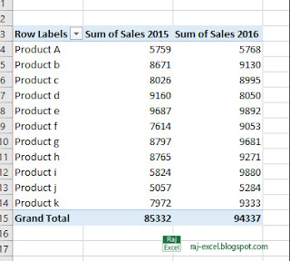
Now in new worksheet you can see some field on the right. Click the Product Field or drag it to Rows area. You will see the product data in first rows. Select sales 2015 and 2016 or drag it to Value area. In Columns area you will see the new field appear automatically when you drag more than one field into Value area.


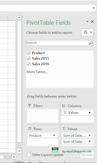
If you have the Area /Zone field, you can drag it to Filter area and you can view the data on Area/Zone level.