Excel Tutorial
Calculate growth formula in pivot table
How to calculate growth formula in PivotTable
Solution of this problem.
Make a pivot table with contain the data 2015 and 2016 sales
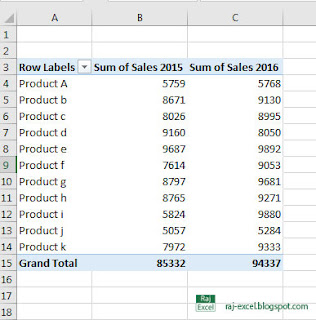
Click anywhere on Pivot Table
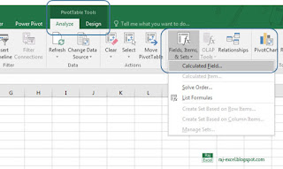
Click the On PivotTable Tools, Analyze Tab, Click the “Fields, Items, & Sets” and then click Calculated Field
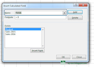
New popup window “Insert Calculated Field” appear on screen
Define the Name: Growth %
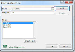
In the area of Formula =
Click the Sales 2016 Fields and click the Insert Field you will see the Formula area after the equel sign “=” Sales 2016 show in Formula area.
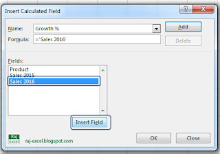
After the selection of Sales 2016 type the “/” divide sign and select the Sales 2015 and click insert field now type % -100 (percentage and minus 100) and then click Add botton.
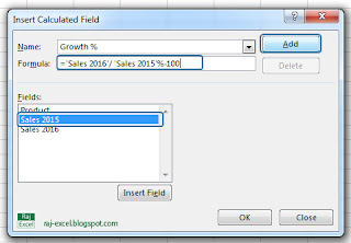
Now you will see the new Field “Growth %” show in Fields area. Click OK
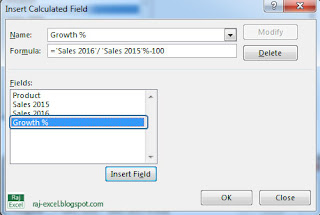
Now you will see the new column inserted in pivot table with the name “Sum of Growth %”
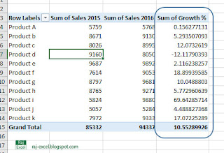
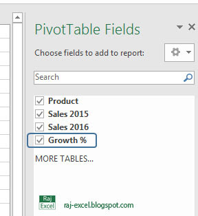
And same will be view “Growth %” in PivotTable Fields.
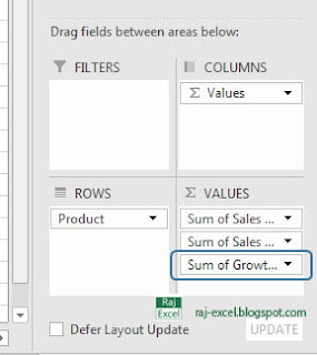
“Sum of Growth%” will also show in Value area in PivotTable Fields
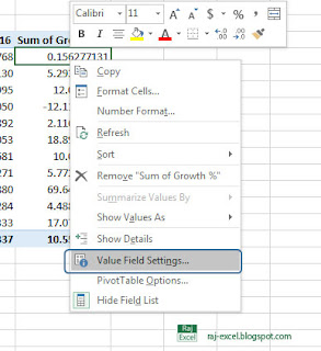
Let’s formatting (Number formatting) – Now format it properly
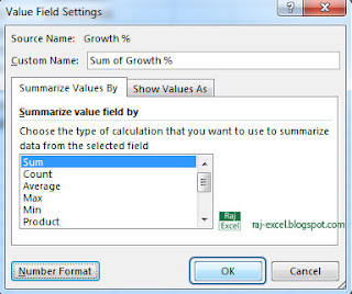
Right click and click the Value Field Settings…
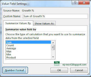
New popup “Value Field Setting” window appear on screen Click the Number Format
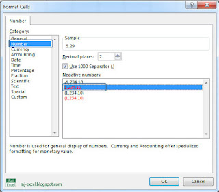
Another popup “Format Cell” appear on screen In Category click the Number and select and define the decimal place in default the decimal places is the 2 (0.00) the Negative number style as you like I selected the second one and click OK
Now again click the OK for “Value Field Settings”
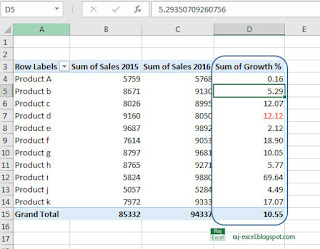
Now you will see the “Growth %” is formatted (Proper number formatting with two decimal).

No comments:
Post a Comment