Excel Functions: AVERAGE()

Excel Function

AVERAGE () Function

Using the AVERAGE Function

Excel Functions: IFNA()

Excel Function

IFNA () Function

Using the IFNA Function

Excel PowerPivot: DATEDIFF Function (DAX)

Excel PowerPivot DAX Function & Features

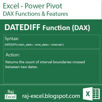
DATEDIFF Function (DAX)

Syntax:

DATEDIFF(<start_date>, <end_date>), <interval>)

Parameters:

start_date: Any DAX expression that returns a datetime value.

end_date: Any DAX expression that returns a datetime value.

interval: The interval to use when comparing dates. The value can be one of the following:

• SECOND

• MINUTE

• HOUR

• DAY

• WEEK

• MONTH

• QUARTER

• YEAR

Action:

Returns the count of interval boundaries crossed between two dates.

 

Excel PowerPivot: CALENDAR Function (DAX)

Excel PowerPivot DAX Function & Features

CALENDAR Function (DAX)

Syntax:

CALENDAR(<start_date>, <end_date>)CALENDAR(<start_date>, <end_date>)

Parameters:

start_date: Any DAX expression that returns a datetime value.

end_date :Any DAX expression that returns a datetime value.

Action:

Returns a table with a single column named “Date” that contains a contiguous set of dates. The range of dates is from the specified start date to the specified end date, inclusive of those two dates.

 

Convert text to Capital-Case (Capitalizes all the letter in Text) in Excel

UPPER function

Capitalizes all the letter and any other letters in text that follow any character other than a letter in a text string. 

Syntax

UPPER(text)

The UPPER function syntax has the following arguments:

• Text    Required. The Text want converted to uppercase. Text can be a reference or text string

Example:

Type your data in C3 cell

and then type the proper function in cell G3

=PROPER(C3)

Here is the result

Convert text to Initial-Case (Capitalizes the first letter in Text) in Excel

PROPER function

Capitalizes the first letter and any other letters in text that follow any character other than a letter in a text string. Converts all other letters in lowercase.

Syntax

PROPER(text)

The PROPER function syntax has the following arguments:

• Text    Required. Text enclosed in quotation marks, a formula that returns text, or a reference to a cell containing the text you want to partially capitalize.

Example:

Type your data in C3 cell

and then type the proper function in cell G3

=PROPER(C3)

Here is the result

Using of SUMIFS function in Excel

SUMIFS function

Adds the cells in a range that meet multiple criteria. For example, if you want to sum the numbers in the range A1:A9 only if the corresponding numbers in B1:B9 are greater than zero (0) and the corresponding numbers in C1:C9 are less than 10, you can use the following formula:

=SUMIFS(A1:A9, B1:B9,"=A*", C1:C9,1)

Find last date of the month in Excel using EOMONTH function

EOMONTH function is to calculate maturity dates or due dates that fall on the last day of the month. It used to return the last day of the month depending on the start date specified.

EMONTH()

Return the serial number of the last day of the month before or after a specified number of months

Syntax:

Note:

If start_date is not a valid date, EOMONTH returns the #NUM! Error value.

If start_date plus months yields an invalid date, EOMONTH returns the #NUM! Error value

Let’s do some task

Date of the last day of the current month, next month last date and previous month last date:

Click the current month last date and type the formula =EMONTH(D5,0). D5 is the current month date and 0 is the number of the month or current month +/-.

Click the Next month last date and type the formula =EMONTH(D5,1). D5 is the current month date and 1 is the number of the month or next month. (Current month plus one month).

Click the Previous month last date and type the formula =EMONTH(D5,-1). D5 is the current month date and -1 is the number of the month or last month (Current month less one month).

For formatting the number convert date (Shortcut Key Ctrl+Shift+$),

Select the cell to display the number as a date, and then on the Home tab, in the Number group, click the arrow next to the Number format and Short Date or click a Long date.

Using LARGE Funtion in Excel

Returns the k-th largest value in a data set. You can use this function to select a value based on its relative standing. For example, you can use LARGE to return the highest, runner-up, or third-place score.
=LARGE(array, k)

The LARGE function syntax has the following arguments:
Array Required. The array or range of data for which you want to determine the k-th largest value.
K Required. The position (from the largest) in the array or cell range of data to return.

Note:

• If array is empty, LARGE returns the #NUM! error value.,
• If k ≤ 0 or if k is greater than the number of data points, LARGE returns the #NUM! error value.

 

 

 

 

 

For example we make a number list that contain 1 to 5 in large function find the largest value after the array or selection you must be define the largest if we type 1 the result appear the first largest data i.e., 5, if we type 2 the result is 2nd largest number i.e, 4.

Function

A prewritten formula that takes a value or values, performs an operation, and returns a value or values. Use functions to simplify and shorten formulas on a worksheet, especially those that perform lengthy or complex calculations.