Automatically update ranking list in Excel

Auto update the ranking list in Microsoft Excel using of INDEX(), MATCH() and LARGE() function

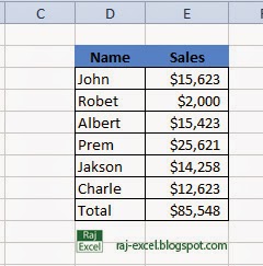
Ok let’s start first we make a list of the employee name with sales value

In routine work everyone use the filter to sort the data using A-Z or Z-A for raking.

If we miss/forget the updating or sort the data and the result is ….?

Let’s make list

And make the list or table with containing Rank, Name and Sales Value column 

Type the rank in ascending order 1 to 6

In cell J3 type the formula =INDEX($D$3:$D$8,MATCH(LARGE($E$3:$E$8,I3),$E$3:$E$8,0))

INDEX(select_ data_name_and_sales)

And select the cell D3 to D8

And type , and start MACH()function, type MATCH(

The match function matching the data from index and the large function select the largest data

MATCH(LARGE(name_list,rank_number),rank_name,0 and close ))

After this now the

=INDEX($D$3:$D$8,MATCH(LARGE($E$3:$E$8,I3)

And see the result

 Copy J3 cell and pate it to J3 to J8

 And now get the sales value data for Prem.

This formula only gets the name rank and now we need the remaining data

Here we can use the VLOOKUP() function

In cell K3 type the formula =VLOOKUP($J3,$D$3:$E$8,2,0)

VLOOKUP(result_of_name_rank, select_ data_name_and_sales,2 second value, 0 and close)

Type K3 =VLOOKUP(select the J3{with $ sing for lock the J Column}

And select the data from D3:E9 {D with $ sing for lock the D Column}

And type after comma 2 {2 is the indicate the second data after the lookup value, if you need the get the data in 3^rd column type 3 instead of 2}

And after the column index just type 0,

 And the result appear in K3 you will see in below picture

And copy the K3 and past it to data as required

The result show in figure below……