Tips of the Day: Microsoft Excel 2013 Short Cut Keys: Alt + HW

Microsoft Excel 2013 Short Cut Keys: Alt + H+W
Hit the Alt key. Then type HW (one key at a time).


Wrap extra-long text into multiple lines so you can see all of it.

raj-excel.blogspot.com (ShortCutKeys)

Tips of the Day: Microsoft Excel 2013 Short Cut Keys: Alt + HAR

Microsoft Excel 2013 Short Cut Keys: Alt + H+A+R
Hit the Alt key. Then type HAR (one key at a time).


Align your content to the right.

raj-excel.blogspot.com (ShortCutKeys)

Tips of the Day: Microsoft Excel 2013 Short Cut Keys: Alt + HAM

Microsoft Excel 2013 Short Cut Keys: Alt + H+A+M
Hit the Alt key. Then type HAM (one key at a time).


Align text so that it is centered between the top and bottom of the cell.

raj-excel.blogspot.com (ShortCutKeys)

Tips of the Day: Microsoft Excel 2013 Short Cut Keys: Alt + HAL

Microsoft Excel 2013 Short Cut Keys: Alt + H+A+L
Hit the Alt key. Then type HAL (one key at a time).


Align your content to the left.

raj-excel.blogspot.com (ShortcutKeys)

Tips of the Day: Microsoft Excel 2013 Short Cut Keys: Alt + HAFR

Microsoft Excel 2013 Short Cut Keys: Alt + H+A+F+R
Hit the Alt key. Then type HAFR (one key at a time).


Set the text to read from right to left.

raj-excel.blogspot.com (Shortcut Keys)

Tips of the Day: Microsoft Excel 2013 Short Cut Keys: Alt + HAFL

Microsoft Excel 2013 Short Cut Keys: Alt + H+A+F+L
Hit the Alt key. Then type HAFL (one key at a time).


Set the text to read from left to right.

raj-excel.blogspot.com (Shortcut keys)

Tips of the Day: Microsoft Excel 2013 Short Cut Keys: Alt + HAFC

Microsoft Excel 2013 Short Cut Keys: Alt + H+A+F+C
Hit the Alt key. Then type HAF (one key at a time).


Allow Excel to choose the paragraph direction based on the language that is being typed.

raj-excel.blogspot.com (Alt+HAFC)

Tips of the Day: Microsoft Excel 2013 Short Cut Keys: Alt + H5

Microsoft Excel 2013 Short Cut Keys: Alt + H+5
Hit the Alt key. Then type H5 (one key at a time).


Move your content closer to the cell border

raj-excel.blogspot.com (Alt+H5)

Add a Secondary axis in a Chart in Microsoft Excel 2013

When the Chart values vary widely from data series to data series, or when you have mixed types of data (for example, units and volume), you can plot one or more data series on a secondary vertical (value) axis. The scale of the secondary vertical axis reflects the values for the associated data series.

After you add a secondary vertical axis to a Clustered column chart, you can also add a secondary horizontal (category) axis, which may be useful in an xy (Line) chart.

To help distinguish the data series that are plotted on the secondary axis, you can change their chart type. For example, in a column chart, you could change the data series on the secondary axis to a line chart.

Type your data as required

Select the data for making the primary chart

 In Microsoft Excel 2013 have only smart tag for some new options, Select the smart tag and click the charts

Select the Clustered Column Chart

When you select he chart the new Chat tab appear on Tab panel go to Design tab and select the chat style as you like

One normal Primary chart is completed

Let’s start to add the Secondary chart

Select the chart anywhere

and right click and Click the Select Data

  After the select Data the new dialog bar popup on screen as show in below figure>

Click the Add button

And select the Series name

In Series name select the Units

And the series values select the Units data Jan to May

And click OK

After the Add a new series the graph is too small because the value of this cart is low as alphabetically.

This second series chart is also part of Primary chat lets change it to Secondary chart

Select the second chat

 .

In Microsoft Excel 2013 the new option of Graph design appear on Right side of Screen

Select the Series Option and Click the Secondary Chat

Now this chart is Secondary chart. Let’s change the chart Type.

Goto Layout Tab and select the Change Chart Type

After you click the Change Chart Type the new dialog box popup the screen. As same shown in picture below.

Drop down box and select the Line Chart 

You can also change the Axis to make a secondary chart just click the check box

 

Now finally this chart have two type of Chart Primary and secondary.

In This chart you will see the two Axis on in Right side and another is on Left side.

In Right side is the Secondary and left side axis for Primary Chart 

And now let’s add the Data Label in both charts

First select he Secondary Chart.

Goto Chart Tool Tab / Design Tab on Left side click the Add Chart Element.

Select he Data Lables and Above.  

And select the Primary Chart

Goto Chart Tool Tab / Design Tab on Left side click the Add Chart Element.

Select he Data Lables and Above. 

And select the Primary Chart

Goto Chart Tool Tab / Design Tab on Left side click the Add Chart Element.

Select he Data Lables and Inside Base. 

And Also inset the legend key in the Chart

Goto Chart Tool Tab / Design Tab on Left side click the Add Chart Element.

Select he Data Table and Select he With Legend Keys. 

And now finally add the chart Title

Goto Chart Tool Tab / Design Tab on Left side click the Add Chart Element.

Select he Chart Title and Select Above Chart. 

  

Let’s link the Chart Title Select the Chart Title and go to formula bar and type the = and using the mouse go to cell C4 select using mouse and click the Enter using the keyboard

Let’s Change the data from general to Accounting type select the data

 Click the comma

And click the less zero

Video Tutorial : Microsoft Excel 2013 Tutorial For Beginners

Microsoft Excel 2013 Tutorial For Beginners #1: Crash Course Data Entry Formulas Formats Charts 365

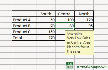
Show the popup text box on cell in Excel 2013

Show the popup text box in cell when you select the cell.

raj-excel.blogspot.com

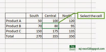
Select the cell you want to appear popup tex box.

raj-excel.blogspot.com

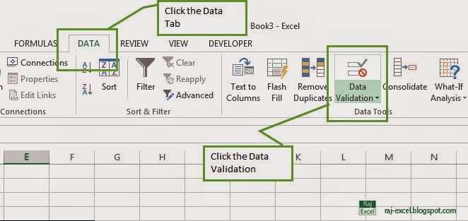
Goto Data tab and click the Data Validation.

raj-excel.blogspot.com

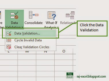
 After the select the Data Validation the drop down tab appear on screen click the Data Validation...

raj-excel.blogspot.com

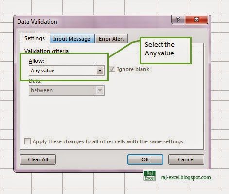
When you click the Data Validation a new dialog box show in screen. In settings tab select the Validation Criteria In Allow drop down box select the Any value.

raj-excel.blogspot.com

 After the selecting of Any value (Don't click the OK button)
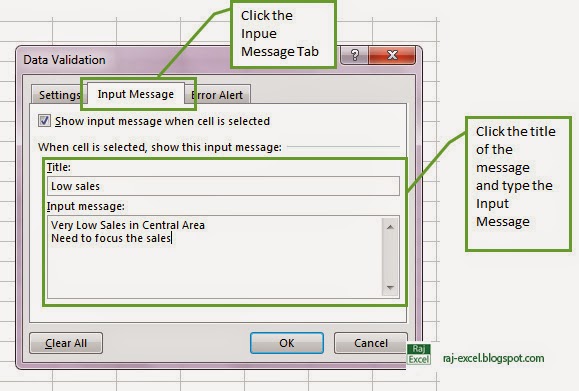
Select the second tab (Input Message) get the check in Show Input message when cell is selected.

and Type the Title of the massage and type your massage in Input Massage box and then click OK.

raj-excel.blogspot.com

raj-excel.blogspot.com